Deep Neural Network from Scratch
Here we will understand the forward pass as well as the backward pass in a Deep neural network .
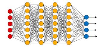 Image credit: [sourced from google]
Import Libraries
import numpy as np
import matplotlib.pyplot as plt
Architecture
steps
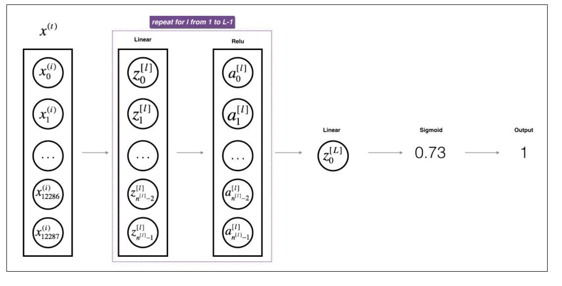
Forward Pass
- initialize parameters (i.e weights & biases)
- caluclate linear forward ( a.k.a Z value)
- calculate linear activation forward ( a.k.a A value)
- calculate forward functions for all L layers
- calculate Cost function
Backward Pass
- calculate linear backward ( a.k.a derivatives)
- calculate linear activation backward
- calculate backward functions for all L layers
- update the parameters (i.e weights & biases)
Forward Pass
Initialize parameters
- Random initialization to weights & zeros to biases
def initialize_parameters_deep(layers_dims):
    """
    Arguments:
    layer_dims -- python array (list) containing the dimensions of each layer in our network

    Returns:
    parameters -- python dictionary containing your parameters "W1", "b1", ..., "WL", "bL":
                    Wl -- weight matrix of shape (layer_dims[l], layer_dims[l-1])
                    bl -- bias vector of shape (layer_dims[l], 1)
    """

    np.random.seed(3)
    parameters={}
    L=len(layers_dims)

    for l in range(1,L):#loop goes from 1 to L-1
        parameters["W"+str(l)]=np.random.randn(layers_dims[l],layers_dims[l-1])*0.01
        parameters["b"+str(l)]=np.zeros((layers_dims[l],1))

        assert(parameters["W"+str(l)].shape == (layers_dims[l], layers_dims[l-1]))
        assert(parameters["b"+str(l)].shape == (layers_dims[l], 1))

    return parameters
layers_dims = np.array([3, 4,4, 1])
parameters = initialize_parameters_deep(layers_dims)
print(parameters)
{'W1': array([[ 0.01788628,  0.0043651 ,  0.00096497],
       [-0.01863493, -0.00277388, -0.00354759],
       [-0.00082741, -0.00627001, -0.00043818],
       [-0.00477218, -0.01313865,  0.00884622]]), 'b1': array([[0.],
       [0.],
       [0.],
       [0.]]), 'W2': array([[ 0.00881318,  0.01709573,  0.00050034, -0.00404677],
       [-0.0054536 , -0.01546477,  0.00982367, -0.01101068],
       [-0.01185047, -0.0020565 ,  0.01486148,  0.00236716],
       [-0.01023785, -0.00712993,  0.00625245, -0.00160513]]), 'b2': array([[0.],
       [0.],
       [0.],
       [0.]]), 'W3': array([[-0.00768836, -0.00230031,  0.00745056,  0.01976111]]), 'b3': array([[0.]])}
Linear Forward
The linear forward module (vectorized over all the examples) computes the following equations:
$$Z^{[l]} = W^{[l]}A^{[l-1]} +b^{[l]}\tag{4}$$ where $A^{[0]} = X$.
def linear_forward(A, W, b):
    """
    Implement the linear part of a layer's forward propagation.

    Arguments:
    A -- activations from previous layer (or input data): (size of previous layer, number of examples)
    W -- weights matrix: numpy array of shape (size of current layer, size of previous layer)
    b -- bias vector, numpy array of shape (size of the current layer, 1)

    Returns:
    Z -- the input of the activation function, also called pre-activation parameter
    cache -- a python tuple containing "A", "W" and "b" ; stored for computing the backward pass efficiently
    """

    Z=np.dot(W,A)+b

    assert(Z.shape ==(W.shape[0],A.shape[1]))
    cache = (A,W,b)

    return Z,cache
Activation functions
def sigmoid(Z):
    Z=np.array(Z)
    return (1/(1+np.exp(-Z)),Z)
sigmoid([[1,2,3],[1,2,3]])
(array([[0.73105858, 0.88079708, 0.95257413],
        [0.73105858, 0.88079708, 0.95257413]]), array([[1, 2, 3],
        [1, 2, 3]]))
def relu(Z):
    Z=np.array(Z)
    return (np.where(Z>0,Z,0),Z)
relu([[1,0.8,-3],[-1,2,0]])
(array([[1. , 0.8, 0. ],
        [0. , 2. , 0. ]]), array([[ 1. ,  0.8, -3. ],
        [-1. ,  2. ,  0. ]]))
Linear activation forward
Sigmoid: $\sigma(Z) = \sigma(W A + b) = \frac{1}{ 1 + e^{-(W A + b)}}$. We have provided you with the sigmoid function. This function returns two items: the activation value “a” and a “cache” that contains “Z” (it’s what we will feed in to the corresponding backward function). To use it you could just call:
A, activation_cache = sigmoid(Z) ReLU: The mathematical formula for ReLu is $A = RELU(Z) = max(0, Z)$. We have provided you with the relu function. This function returns two items: the activation value “A” and a “cache” that contains “Z” (it’s what we will feed in to the corresponding backward function). To use it you could just call:
A, activation_cache = relu(Z)
def linear_activation_forward(A_prev, W, b, activation):
    """
    Implement the forward propagation for the LINEAR->ACTIVATION layer

    Arguments:
    A_prev -- activations from previous layer (or input data): (size of previous layer, number of examples)
    W -- weights matrix: numpy array of shape (size of current layer, size of previous layer)
    b -- bias vector, numpy array of shape (size of the current layer, 1)
    activation -- the activation to be used in this layer, stored as a text string: "sigmoid" or "relu"

    Returns:
    A -- the output of the activation function, also called the post-activation value
    cache -- a python tuple containing "linear_cache" and "activation_cache";
             stored for computing the backward pass efficiently
    """

    if activation=='sigmoid':
        Z,linear_cache = linear_forward(A_prev, W, b)
        A , activation_cache = sigmoid(Z)

    if activation=='relu':
        Z,linear_cache = linear_forward(A_prev, W, b)
        A ,activation_cache = relu(Z)

    assert (A.shape == (W.shape[0], A_prev.shape[1]))
    cache = (linear_cache, activation_cache)

    return A, cache
L Model forward
def L_model_forward(X, parameters):
    """
    Implement forward propagation for the [LINEAR->RELU]*(L-1)->LINEAR->SIGMOID computation

    Arguments:
    X -- data, numpy array of shape (input size, number of examples)
    parameters -- output of initialize_parameters_deep()

    Returns:
    AL -- last post-activation value
    caches -- list of caches containing:
                every cache of linear_activation_forward() (there are L-1 of them, indexed from 0 to L-1)
    """
    AL=[]
    A=X
    caches=[]
    L=len(parameters)//2

    for l in range(1,L):

        A_prev =A

        A, cache = linear_activation_forward(A_prev,parameters["W"+str(l)],parameters["b"+str(l)],"relu")
        caches.append(cache)


    AL , cache=linear_activation_forward(A,parameters["W"+str(L)],parameters["b"+str(L)],"sigmoid")
    caches.append(cache)

    assert(AL.shape ==(1,X.shape[1]))
    return AL,caches
Cost Function
def compute_cost(AL,Y):
    """
    Implement the cost function defined by equation (7).

    Arguments:
    AL -- probability vector corresponding to your label predictions, shape (1, number of examples)
    Y -- true "label" vector (for example: containing 0 if non-cat, 1 if cat), shape (1, number of examples)

    Returns:
    cost -- cross-entropy cost
    """
    m = Y.shape[1]

    cost = -1/m*np.sum(Y*np.log(AL)+(1-Y)*np.log((1-AL)))


    cost = np.squeeze(cost) # To make sure your cost's shape is what we expect (e.g. this turns [[17]] into 17).
    assert(cost.shape == ())

    return cost
Backward Pass
Linear Backward
For layer $l$, the linear part is: $Z^{[l]} = W^{[l]} A^{[l-1]} + b^{[l]}$ (followed by an activation).
Suppose you have already calculated the derivative $dZ^{[l]} = \frac{\partial \mathcal{L} }{\partial Z^{[l]}}$. You want to get $(dW^{[l]}, db^{[l]}, dA^{[l-1]})$.
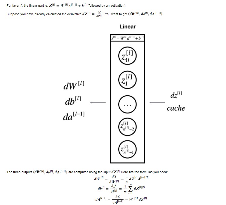
The three outputs $(dW^{[l]}, db^{[l]}, dA^{[l-1]})$ are computed using the input $dZ^{[l]}$ (using formulae above).
def linear_backward(dZ,cache):
    """
    Implement the linear portion of backward propagation for a single layer (layer l)

    Arguments:
    dZ -- Gradient of the cost with respect to the linear output (of current layer l)
    cache -- tuple of values (A_prev, W, b) coming from the forward propagation in the current layer

    Returns:
    dA_prev -- Gradient of the cost with respect to the activation (of the previous layer l-1), same shape as A_prev
    dW -- Gradient of the cost with respect to W (current layer l), same shape as W
    db -- Gradient of the cost with respect to b (current layer l), same shape as b
    """
    A_prev, W, b = cache
    m = A_prev.shape[1]

    dW = 1/m*np.dot(dZ,A_prev.T)
    db =1/m*np.sum(dZ,axis=1,keepdims=True)
    dA_prev =np.dot(W.T,dZ)

    assert(dA_prev.shape == A_prev.shape)
    assert(dW.shape == W.shape)
    assert(db.shape == b.shape)

    return dA_prev, dW, db
Backward activation functions
def sigmoid_backward(dA, activation_cache):
    """
    activation_cache= Z
    """
    Z=np.array(activation_cache)
    val=1/(1+np.exp(-Z))
    return (dA*val*(1-val))
sigmoid_backward([[1,2,3],[1,2,3]],[[1,2,3],[1,2,3]])
array([[0.19661193, 0.20998717, 0.13552998],
       [0.19661193, 0.20998717, 0.13552998]])
def relu_backward(dA, activation_cache):
    """
    activation_cache= Z
    """
    Z=np.array(activation_cache)
    return (dA*np.where(Z>0,1,0))
relu_backward([[1,2,3],[1,2,3]],[[1,0.8,-3],[-1,2,0]])
array([[1, 2, 0],
       [0, 2, 0]])
Linear activation backward
To help implement linear_activation_backward, we provided two backward functions:
sigmoid_backward: Implements the backward propagation for SIGMOID unit. You can call it as follows: dZ = sigmoid_backward(dA, activation_cache) relu_backward: Implements the backward propagation for RELU unit. You can call it as follows: dZ = relu_backward(dA, activation_cache) If $g(.)$ is the activation function, sigmoid_backward and relu_backward compute$$dZ^{[l]} = dA^{[l]} * g'(Z^{[l]}) \tag{11}$$
def linear_activation_backward(dA, cache, activation):
    """
    Implement the backward propagation for the LINEAR->ACTIVATION layer.

    Arguments:
    dA -- post-activation gradient for current layer l
    cache -- tuple of values (linear_cache, activation_cache) we store for computing backward propagation efficiently
    activation -- the activation to be used in this layer, stored as a text string: "sigmoid" or "relu"

    Returns:
    dA_prev -- Gradient of the cost with respect to the activation (of the previous layer l-1), same shape as A_prev
    dW -- Gradient of the cost with respect to W (current layer l), same shape as W
    db -- Gradient of the cost with respect to b (current layer l), same shape as b
    """
    linear_cache, activation_cache = cache

    if activation == "sigmoid":
        dZ =sigmoid_backward(dA, activation_cache)
        dA_prev, dW, db = linear_backward(dZ, linear_cache)

    elif activation == "relu":
        dZ = relu_backward(dA, activation_cache)
        dA_prev, dW, db = linear_backward(dZ, linear_cache)

    return dA_prev, dW, db
L model backward
def L_model_backward(AL, Y, caches):
    """
    Implement the backward propagation for the [LINEAR->RELU] * (L-1) -> LINEAR -> SIGMOID group

    Arguments:
    AL -- probability vector, output of the forward propagation (L_model_forward())
    Y -- true "label" vector (containing 0 if non-cat, 1 if cat)
    caches -- list of caches containing:
                every cache of linear_activation_forward() with "relu" (it's caches[l], for l in range(L-1) i.e l = 0...L-2)
                the cache of linear_activation_forward() with "sigmoid" (it's caches[L-1])

    Returns:
    grads -- A dictionary with the gradients
             grads["dA" + str(l)] = ...
             grads["dW" + str(l)] = ...
             grads["db" + str(l)] = ...
    """
    grads = {}
    L = len(caches) # the number of layers
    m = AL.shape[1]
    Y = Y.reshape(AL.shape)# after this line, Y is the same shape as AL

    # Initializing the backpropagation
    dAL = - (np.divide(Y, AL) - np.divide(1 - Y, 1 - AL))

    ###Lth layer (SIGMOID -> LINEAR) gradients. Inputs: "dAL, current_cache".
    ###Outputs: "grads["dAL-1"], grads["dWL"], grads["dbL"]
    current_cache = caches[L-1]
    grads["dA" + str(L-1)], grads["dW" + str(L)], grads["db" + str(L)] =linear_activation_backward(dAL, current_cache, "sigmoid")

    # Loop from l=L-2 to l=0
    for l in reversed(range(L-1)):
        # lth layer: (RELU -> LINEAR) gradients.
        # Inputs: "grads["dA" + str(l + 1)], current_cache".
        ###Outputs: "grads["dA" + str(l)] , grads["dW" + str(l + 1)] , grads["db" + str(l + 1)]
        ### START CODE HERE ### (approx. 5 lines)
        current_cache =caches[l]
        dA_prev_temp, dW_temp, db_temp =linear_activation_backward(grads["dA" + str(l+1)], current_cache, activation = "relu")
        grads["dA" + str(l)] = dA_prev_temp
        grads["dW" + str(l + 1)] = dW_temp
        grads["db" + str(l + 1)] =db_temp

    return grads
Update Parameters
update the parameters of the model, using gradient descent:
$$ W^{[l]} = W^{[l]} - \alpha \text{ } dW^{[l]} $$$$ b^{[l]} = b^{[l]} - \alpha \text{ } db^{[l]} $$ where $\alpha$ is the learning rate. After computing the updated parameters, store them in the parameters dictionary.
Implement update_parameters() to update your parameters using gradient descent.
def update_parameters(parameters, grads, learning_rate):

    L = len(parameters) // 2 # number of layers in the neural network

    # Update rule for each parameter.

    for l in range(L):
        parameters["W" + str(l+1)] = parameters["W" + str(l+1)]-learning_rate*grads["dW" + str(l+1)]
        parameters["b" + str(l+1)] =  parameters["b" + str(l+1)]-learning_rate*grads["db" + str(l+1)]


    return parameters
L-layer neural network(Final)
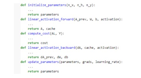
Question: Use the helper functions you have implemented in the previous assignment to build a 2-layer neural network with the following structure: LINEAR -> RELU -> LINEAR -> SIGMOID. The functions you may need and their inputs are:
def L_layer_model(X, Y, layers_dims, learning_rate = 0.0075, num_iterations = 3000, print_cost=False):
"""
Implements a L-layer neural network: [LINEAR->RELU]*(L-1)->LINEAR->SIGMOID.
Arguments:
X -- data, numpy array of shape (num_px * num_px * 3, number of examples)
Y -- true "label" vector (containing 0 if cat, 1 if non-cat), of shape (1, number of examples)
layers_dims -- list containing the input size and each layer size, of length (number of layers + 1).
learning_rate -- learning rate of the gradient descent update rule
num_iterations -- number of iterations of the optimization loop
print_cost -- if True, it prints the cost every 100 steps
Returns:
parameters -- parameters learnt by the model. They can then be used to predict.
"""
np.random.seed(3)
costs = [] # to keep track of the cost
# Initialize parameters dictionary
parameters = initialize_parameters_deep(layers_dims)
# Loop (gradient descent)
for i in range(0, num_iterations):
# Forward propagation:
#[LINEAR -> RELU]*(L-1) -> LINEAR -> SIGMOID.
AL, caches = L_model_forward(X, parameters)
# Compute cost
cost = compute_cost(AL, Y)
# Backward propagation.
grads = L_model_backward(AL, Y, caches)
# Update parameters.
### START CODE HERE ### (approx. 1 line of code)
parameters = update_parameters(parameters, grads, learning_rate)
if print_cost and i % 100 == 0:
print("Cost after iteration {}: {}".format(i, np.squeeze(cost)))
if print_cost and i % 100 == 0:
costs.append(cost)
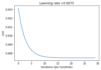
plt.plot(np.squeeze(costs))
plt.ylabel('cost')
plt.xlabel('iterations (per hundreds)')
plt.title("Learning rate =" + str(learning_rate))
plt.show()
return parameters
Implement 4-layer neural network
layers_dims = ([3,4,5,2,1])
X=np.random.randn(3,150)
Y=[]
for i in range(150):
    Y.append(np.random.randint(0,2))
Y=np.array(Y)
Y=np.reshape(Y,(1,150))
print(X.shape,Y.shape)
(3, 150) (1, 150)
L_layer_model(X, Y, layers_dims, learning_rate = 0.0075, num_iterations = 3000, print_cost=True)
Cost after iteration 0: 0.693147179101668
Cost after iteration 100: 0.6913663615472958
Cost after iteration 200: 0.6901428329273512
Cost after iteration 300: 0.6893019578750604
Cost after iteration 400: 0.6887238512106988
.
.
.
.
.
.
Cost after iteration 2700: 0.6874476979055951
Cost after iteration 2800: 0.6874476213206875
Cost after iteration 2900: 0.6874475684872733
 #looking at the parameters learnt
{'W1': array([[ 0.01788646,  0.00436687,  0.00096225],
        [-0.01863628, -0.00277482, -0.00354674],
        [-0.00082677, -0.00627067, -0.00043808],
        [-0.00476898, -0.01314048,  0.00884857]]),
 'b1': array([[-2.64082146e-07],
        [ 2.72834707e-07],
        [ 3.64257323e-07],
        [ 1.75856439e-06]]),
 'W2': array([[ 0.0088149 ,  0.01709711,  0.00049992, -0.00404753],
        [-0.0054536 , -0.01546477,  0.00982367, -0.01101068],
        [-0.01185051, -0.00205634,  0.01486141,  0.00236701],
        [-0.01023786, -0.00712985,  0.00625262, -0.00160502],
        [-0.00768738, -0.00230125,  0.00745106,  0.01976248]]),
 'b2': array([[ 2.34080642e-05],
        [ 0.00000000e+00],
        [-2.81738458e-06],
        [ 1.85347160e-05],
        [ 8.13445992e-05]]),
 'W3': array([[-0.01244123, -0.00626417, -0.00803766, -0.02419083, -0.00923792],
        [-0.01024285,  0.01123978, -0.00131827, -0.01623289,  0.0064712 ]]),
 'b3': array([[0.        ],
        [0.00374547]]),
 'W4': array([[-0.00356271, -0.01783282]]),
 'b4': array([[-0.21327127]])}